Thursday, 7 December 2017

Export data from SQL database into Microsoft Excel 2016

Hi all
This post is in continuation of previous post where sensor data is stored in SQL database over Microsoft Azure. Sometimes, we want to process our data offline for which we may need to fetch the data from SQL server and store in Excel or CSV format. So, in that situation, we need to export data stored in SQL database into Microsoft Excel 2016 format for offline processing. 
Here are the steps to do it:
·       Open New Excel Sheet
·       Click on Data Header, Get Data—From Database—From SQL server database
·       It will ask from SQL server address. This address is available in Microsoft Azure portal, in sql database—overview—server name. For my project, address is: azuredisonsqlserver.database.windows.net
·       For the first time, it may give error for connection. You have to allow it in Azure firewall.
·       In Sql database—overview option, Click on Set Server Firewall option—Click Add Client IP. Make sure that Microsoft Azure and Microsoft Excel is on same network.
·       Now try to open SQL database in Microsoft Excel.
·       It would open Navigator page, which would have Display Options like this:


·       Select AzureEdison Table and click Load option available at bottom. This step would import your data from SQL server available in Microsoft Azure into Microsoft Excel.
·       Now you can do any processing in your data offline also. 
     
      Happy learning and please post your comments below:-)


Reading Sensor data and uploading it on Microsoft Azure

Reading Sensor data via Intel Edison and storing data in SQL database over Microsoft Azure 


  • In this post, I have explained the entire process in bullet points. In this project, using Ambient light sensor, the sensor value is displayed on terminal console, which is actually sent at Microsoft Azure. 
  • This value can be verified using Device Explorer tool, Later Using Stream Analytics Job, the data is streamed and saved in SQL server, which is created online, in Microsoft Azure in form of SQL table. At this stage, this data can be used for analysis purpose and data visualization using suitable tools such as Power BI.


-- Open portal.azure.com
-- Click New—Internet of Things—IoT Hub
-- Give unique name to your IoT hub –Select pricing to Free –resource group (create new and give any name) and create it.
-- Now go to Dashboard and click on you newly create IoT Hub.
-- Go to Settings—Shared Access Policies—select policy “IoT Hub Owner”—Go to Shared access key—Select “Connection String—primary key” and copy the key. And paste it in notepad. This is Key 1.
-- In Iot hub, search for IoT Devices, click on “Add”, give device id, authentication type—symmetric key, select auto generate key, Enable with connect device to IoT Hub and Save. 
-- After Save, reopen the device and copy Connection String--Primary key in notepad. This is Key 2.

-- Go to this page to download “Device Explorer” https://github.com/Azure/azure-iot-sdk-csharp/releases and then install it.
-- Paste the copied connection string (Key 1) in box under configuration tab –IoT Hub Connection String and Update.
-- Click on Management tab and click create tab—give name to Device ID.
-- Once it is created, a device id with given name is create with multiple tabs.
-- Click under Connection string Tab, right click on content—copy connection string for selected device and paste it again in notepad. This is the same key 2 you got earlier also.
Paste this key in program against connectionString variable.
-- This key is very essential for sending data to Microsoft Azure IoT Hub.


Actual program which would run in Edison, written in JavaScript (This program will fetch light intensity and post that data via MQTT protocol usingg Microsoft Azure IoT Hub)


var mraa = require("mraa") ;
var sense= new mraa.Aio(0);
var Protocol = require('azure-iot-device-mqtt').Mqtt;
var Client = require('azure-iot-device').Client;
var Message = require('azure-iot-device').Message;

//
//Azure methods
//
var connectionString=”HostName=azuredison.azure-devices.net;DeviceId=azuredison_iot;SharedAccessKey=xxxxxxxxxxxxxxxxxxxxxx”;
var client = Client.fromConnectionString(connectionString, Protocol);
var connectCallback = function (err) {
  if (err) {
    console.error('Could not connect: ' + err.message);
  } else {
    console.log('Client connected');
    client.on('message', function (msg) {
      console.log('Id: ' + msg.messageId + ' Body: ' + msg.data);
      client.complete(msg, printResultFor('completed'));
    });

  }
};
client.open(connectCallback);

function lightRead()
{
    var lightVal= sense.read();
    //console.log(lightVal);
    var obj= {"lightVal":lightVal};
    var json= JSON.stringify(obj);
    var message = new Message(json);
    client.sendEvent(message, printResultFor('send'));
    console.log(json);
    setTimeout(lightRead,10000);
}
lightRead();
function printResultFor(op) {
  return function printResult(err, res) {
    if (err) console.log(op + ' error: ' + err.toString());
    if (res) console.log(op + ' status: ' + res.constructor.name);
  };
}


·       Access Intel Edison using Putty/TeraTerm and install following packages in Intel Edison (Yocto Linux)
#                              npm install azure-iot-device-mqtt
                                npm install azure-iot-device
  -- Paste connection String copied in notebook in connection string variable. 
  -- Run this code and it will through light intensity values on console
  -- Go to device Explorer tool—Data Tab—Select Device ID as created—Click Monitor Tab.
  -- You should be able to see the light intensity data in this tool. This means that data is transferred to Microsoft Azure But we are able to check its value in this tool.
  -- Click on New—SQL Database—Create
  -- Give Name to SQL database—Subscription—Free Trial—Resource Group—Use existing—Blank Database—Create new sql server—give server name, usename and password for sql server.
  -- After sql database is created, Goto Data explorer (preview) option, login to sql server, and run Query. This query would create sql table where variable LightVal data would be stored:
                    create table AzureIoTEdison(LightVal varchar(255));   
   
  -- Run another query. This query would fetch all data stored in sql table AzureIoTEdison. Since at this stage no value is available (program is not running in edison), it would return 0:
                     Select * from AzureIoTEdison
  
  -- Click New—Search Stream Analytics Job—Create. Click on overview window and look in Job Topology.
  -- There three blocks are available: Inputs, Query, Output.
  -- Click on Input Block—Add—Input alias—“Edison” or any name of input device. Source—IoT Hub.
  -- IoT hub—selected automatically, Event serialization format—JSON, Encoding—UTF-8
  -- Click Create
  -- Click on Output Block—Add—Give output alias name—Edisonoutputdata. Sink—SQL database, Database—selected automatically, give username & password for SQL database, Table—AzureIoTEdison (name of the table created)--Click Create
  
  -- Click on Query Block. Paste this code :

          SELECT
    lightVal
INTO
    [edisonoutputdata]
FROM
    [edison]

Save

-- Start Stream Job
-- Run the code in Edison using Putty #node main.js
-- Open Device Explorer tool

-- Open new tab and open portal.azure.com here again

-- Open dashboard, sql database, Data Explorer(preview)—login to sql server and type query and run:
                    Select * from AzureEdison
-- Now in the result window of sql sever, you can see the data coming up from sensor.  
-- Same data is also visible in Data Explorer tool. This data also get stored in SQL Database. Make sure your program is already running in Edison.
-- In Sql database, in DatExplore(preview) option, login to sql server. You will see multiple options as: Tables, Views, Stored Procedures.
-- Click on Tables—dbo.AzureIoTEdison—LightVal(varchar,null). This is the table in which sensor data is stored in SQL server. TO view this data, Select dbo.AzureIoTEdison—Click Edit Data(Preview). You can map these values with the values generated by sensors in Putty Console or Data Explorer. This verifies that Data actually get stored in SQL server in Microsoft Azure cloud.
-- Once you are done, you can Stop Stream Analytics Job.
Hope you have got a fair insight of how to save sensor data in SQL database over Microsoft Azure. Steps mentioned in this post are well verified and tested,still, if you face any issue, feel free to post your query. I would be happy to help you.
I will come up with few more interesting posts on Microsoft Azure in coming future.

Stay tuned and post your comments!

Python Programming for Data Analytics: Pandas library Basics

Pandas Library
pandas is an open source, BSD-licensed library providing high-performance, easy-to-use data structures and data analysis tools for the Python programming language.
Importing panda library
import pandas as pd

Convert list elements into series of elements ranging from 10—50
import numpy as np
import pandas as pd
my_data=[10,20,30,40,50]
pd.Series(data=my_data)           
# convert element lists into series of elements, which have index from 0—5

Convert dictionary values into series of elements ranging from 10—50
import numpy as np
import pandas as pd
d={'a':10,'b':20,'c':30,'d':40}     
#dictionary keys act as index and values with every key act as series values
pd.Series(d)

Addition of two series
import numpy as np
import pandas as pd
ser1=pd.Series([1,2,3,4],['USA','Germany','Japan','USSR’])  
#create series from 1—4 with index as country names
ser2=pd.Series([1,2,5,4],['USA','Germany','Italy','USSR’])
ser1+ser2 
#addition of 2 series; values get added where index match but if same index is not available in either of series, it generates NaN value

Generate 5x4 table filled with random values having labels for rows and columns (similar to dataset) and pick a particular columns for processing.
from numpy.random import randn
import pandas as pd
np.random.seed(101)
df=pd.DataFrame(randn(5,4),['A','B','C','D','E'],['W','X','Y','Z’]) 
#generate random number for 5 rows and 4 columns, row labels: A—E, columns labels: W—Z. 
df
df[‘W’]
df[[‘W’,’Z’]]

Modifying datasets using panda library

df.drop('W',axis=1,inplace=True)                          
#Droping selected column from dataset; inplace=True, permanently accepts modification
df.loc['A']                          # rows are also series; fetch particular row from dataset having index ‘A’
df.iloc[3]                           # fetch 3rd row from dataset
df.loc[['A','C'],['X','Z’]]                  #fetch a subset of data from given dataset; [[row][column]]
df > 0                                 # all those locations in dataset which are less than threshold is taken False
df[df>0]                            #all those positions in datasets which are less than threshold is taken as NaN
df=pd.DataFrame(randn(5,4),['A','B','C','D','E'],['W','X','Y','Z’]) 
df[df['W']>0]                   
#Select the row where True is available in W column and fetch other elements in same row
df[df['W']>0][['X','Y']]                  
# fetch out desired frame of X & Y from dataset, for those rows where value is more than 0 in ‘W’ column;
df.reset_index()   #assign natural index
df.set_index(‘Z’)    #set ‘Z’ column as index value

Drop missing elements from dataset
import pandas as pd
d={'A':[1,2,np.NaN], 'B':[1,np.NaN,np.NaN],'C':[1,2,3]}    
# np.NaN is the missing element in DataFrame
df=pd.DataFrame(d)
df.dropna()                                     #pandas would drop any row with missing value
df.dropna(axis=1)                          #drop column with NULL value
df.dropna(thresh=2)      
#thresh is the variable for threshold which says that it would not drop row until unless it has atleast 2 NonNA values else it would drop row.

Filling suitable value instead of NaN in dataset
df.fillna(value='FILL VALUE')                      #NaN is replaced by value=FILL VALUE
df['A'].fillna(value=df['A'].mean())    
#Select column "A" and fill the missing value with mean value of the column A

Calculating mean and standard deviation on values in given dataset

data = {'Company':['GOOG','GOOG','MSFT','MSFT','FB','FB'],        #create temporary dataset
'Person':['Sam','Charlie','Amy','Vanessa','Carl','Sarah'],
'Sales':[200,120,340,124,243,350]}
df=pd.DataFrame(data)               #connect data as dataframe which have row and column label
df
comp=df.groupby("Company").mean() 
# data in dataset is grouped by label “Company” i.e. elements with similar company names are grouped together and after grouping data, aggregate ‘mean’ function is applied on its value; mean could not be applied on second column "person name" due to string type
comp
comp1=df.groupby("Company")              #grouping done using label name “Company”
comp1.std()                                                  #apply standard deviation on grouped data

Fetching particular data from dataset after applying aggregate function

data = {'Company':['GOOG','GOOG','MSFT','MSFT','FB','FB'],        #create temporary dataset
'Person':['Sam','Charlie','Amy','Vanessa','Carl','Sarah'],
'Sales':[200,120,340,124,243,350]}
df=pd.DataFrame(data)               #connect data as dataframe which have row and column label
df.groupby("Company").sum().loc["FB"]              
#group data by ‘company’ label, apply sum function such that all data of same company gets added and then fetch Company “FB” value after summation

Finding maximum value in each label in dataset
data = {'Company':['GOOG','GOOG','MSFT','MSFT','FB','FB'],        #create temporary dataset
'Person':['Sam','Charlie','Amy','Vanessa','Carl','Sarah'],
'Sales':[200,120,340,124,243,350]}
df=pd.DataFrame(data)               #connect data as dataframe which have row and column label
df.groupby("Company").max()  
#group dataset based on ‘company’ label and pick maximum value in each label

Find unique value and number of occurrence of values in dataset

df = pd.DataFrame({'col1':[1,2,3,4],'col2':[444,555,666,444],'col3':['abc','def','ghi','xyz’]})
# col1, col2 & col3 are column labels, each column have their own values
df['col2'].unique()           #fetches the unique values available in column ‘col2’
df['col2'].value_counts()             
# count number of occurance of every value in column and display its count

Save Data frame into CSV file or Excel file
df.to_csv('example.csv',index=False)

df.to_excel('Excel_Sample.xlsx',sheet_name='Sheet1')

Hope you have enjoyed doing basic Data Munging with Pandas Libraries. 

Stay Calm and learn. Please post your comments below :-) 

Python Programming for Data Analytics: Matplotlib library Basics

Matplotlib Tool
Matplotlib is a plotting library for the Python programming language and its numerical mathematics extension NumPy. It provides an object-oriented API for embedding plots into applications using general-purpose GUI toolkits like TKinter, wxPython, Qt, or GTK+.
Source: Wikipedia

Importing matplotlib and numpy to plot line graph
import matplotlib.pyplot as plt
%matplotlib inline
import numpy as np
x = np.linspace(0, 5, 11)               #generate 1D array starting from 0—5, total 11 elements
y = x ** 2                                         # x2
plt.plot(x, y, 'r’)                              # 'r' is the color red
plt.xlabel('X Axis Title Here')                      #label x asis
plt.ylabel('Y Axis Title Here')                      # label y axis
plt.title('String Title Here')                         # give title to plot
plt.show()                                                     # show plot

Create subplot in single plot (like MATLAB)
plt.subplot(1,2,1)                          # 1 row, 2 columns, 1st figure in row
plt.plot(x, y, 'r--')                            # r—red color, -- for dashed graph lines
plt.subplot(1,2,2)                          # 1 row, 2 columns, 2nd figure in row
plt.plot(y, x, 'g*-');                         # g—green color, *- for graph lines

Use subplot functions to create MATLAB style line color
import matplotlib.pyplot as plt
%matplotlib inline
import numpy as np
x = np.linspace(0, 5, 11)
fig, ax = plt.subplots()                              #generate 2 objects, fig and ax
ax.plot(x, x**2, 'b.-')                               # blue line with dots
ax.plot(x, x**3, 'g--')                              # green dashed line
ax.set_xlabel('x axis’)
ax.set_ylabel('y axis')
ax.set_title(' plot title')

Plot various types of plots (scatter, step, bar and fill) in same figure
import numpy as np
import matplotlib.pyplot as plt
%matplotlib inline

n = np.array([0,1,2,3,4,5])
xx = np.linspace(-0.75, 1., 100)
fig, axes = plt.subplots(1, 4, figsize=(12,3))        #create figure of dimension 12x3 inch, with 4 subplots
axes[0].scatter(xx, xx + 0.25*np.random.randn(len(xx)))
axes[0].set_title("scatter")
axes[1].step(n, n**2, lw=2)                       #lw=line width of 2
axes[1].set_title("step")
axes[2].bar(n, n**2, align="center", width=0.5, alpha=0.5)     #alpha – transparency level
axes[2].set_title("bar")
axes[3].fill_between(xx, xx**2, xx**3, color="green", alpha=0.5);
axes[3].set_title("fill_between");

Saving plot into file format
fig.savefig("filename.png")

fig.savefig("filename.png", dpi=200)

Hope you have enjoyed working with Matplotlib library and plotted beautiful graphs of your data :-)
In next post, I would come up with another popular and important library used for Data Analytics purpose. 
Keep learning.Keep Growing :-) Please post your comments below !

Python Programming for Data Analytics: NumPy Library Basics

NumPy Library
NumPy is the core library for scientific computing in Python. It provides a high-performance multidimensional array object, and tools for working with these arrays.

Create 2-D array using numpy from list
import numpy as np
mylist=[[1,2,3],[4,5,6],[7,8,9]]
np.array(mylist)

Create 1-D and 2-D array using random values
np.random.rand(5)             #uniform distribution of random values
np.random.rand(4,4)          # create 2-D array of random values
np.random.randn(4)        #std. normal distribution, centered around 0

Fetch Max on Min value from array
arr1=np.random.randint(0,100,10)    #10 random integer elements
arr1.max()    or arr1.min()

Playing with the data using numpy library
arr=np.arange(0,11)                            #create array of 10 elements between 1—10
arr[:5]                                                 #fetch 1st 5 elements of array arr
arr[5:]                                                  #fetch elements from 5th positions till last elements
arr[:2]=100                                        # replace the 1st two elements of array with value 100
arr=np.arange(0,25)
arr.reshape(5,5)                                             #reshape method which reshapes 1-D array into 2-D array
arr_2d=np.array([[1,2,3],[4,5,6],[7,8,9]])     #create 2-D array
arr_2d[:2,1:]                                              # select elements in a particular row and column in 2D array
arr=np.arange(0,11)
arr > 5                                                        #return True for elements position which is more than 5
arr[arr<5]                        
# return True for elements position which is more than 5 and pick array values for True positions
arr+arr                                                       # element by element array addition
mat = np.arange(1,26).reshape(5,5)    #generate 1D array of 15 elements and convert it into 2D array
mat.std()                                     #finding standard deviation on elements

mat.sum(axis=0)                        #summing elements column wise in given array mat

Hope you had enjoyed working with these basics of NumPy library. in next post, I would come up with another popular library used in Data Analytics.

Happy Learning! Please post your comments below :-)
Wednesday, 16 August 2017

Flashing Intel Edison Firmware Manually

Hello everyone
Generally, we flash Intel Edison Boards with Intel Edison Board Configuration Tool on Windows 10/Windows 7. But, sometimes,while we are flashing the Yocto Linux Image on Edison board, it fails!!. At that time, we must do a manual flash of image.

Open Windows command prompt for manual installation.Go to folder where image is available, unpack the image, download “dfu-util-0.9” or latest version for windows from given link, download dfu-util-0.9-win64.zipextract file “dfu-util” and “libusb-1.0.dll” and paste in the same folder of image.
Now, using command prompt, go the directory where the extracted image was stored, run “flashall.bat” on command prompt. It should come like this:


·         Once It is done, do not immediately remove cable. Leave it for 2-4 min. Disconnect the board and again open the Intel Edison Board Configuration Tool. This time, the Firmware option in tool must be green which signifies that board is successfully installed with latest firmware.


·         If by any case, Firmware/Image does not get installed (still yellow color) in this method, Firmware might have got corrupted and re-flash need to be done. In such case, we should take few extra steps:

      1. Connect board to laptop, access board using Teraterm/Putty/MobaXTerm using COM USB.
      2. Set Serial Baud rate to 115200 and boot board with existing firmware.
      3. When you come across following message, press key to enter in boot mode


      Stop the autoboot process on the Edison and get the the "boot >" prompt. Once you're at the "boot >" prompt, type "run do_flash". You should see the following output:
      Saving Environment to MMC...
      Writing to redundant MMC(0)... done
      GADGET DRIVER: usb_dnl_dfu
      Once you see the "GADGET DRIVER: usb_dnl_dfu" message, the Edison board is in the correct state to accept flashing again. 

       Now use, windows command prompt to reach to the directory where extracted Yocto image is placed  and files “dfu-util” and “libusb-1.0.dll” are copied and pasted as explained in beginning of post. Run  from the following command "flashall.bat". This would re-flash your firmware from beginning and make  your board re-usable. 

      This is tried and tested method and gives 100% result... Try for yourself !
       Happy Learning :-)

Monday, 7 August 2017

Role of APIs, System calls & Device Drivers explained with example

Here, we are going to talk about API, System calls and device drivers. Lets start with API first.

API (Application Programming Interface): API are the functions or entry points provided by any application or system to use its features. Application developer need not to reinvent the wheel, he just uses the API available and manage to use the feature of different applications in his own application.ex. using Google map API in your application to identify location for given latitude and longitude.
From system perspective, application developer uses the system API to access certain features or resources provided by system in simplified manner. Application developer need not to develop the process or method to access the system so his job is simplified and fast. ex. accessing ram space by any application

System calls: System calls are the entry point to kernel space so that any application can talk to kernel and make it understand what is needed by them.ex. we can use google apis to access location in any application but sohow this intend is to told to kernel so that it can further talk to processor about same and make hardware work for application requirements. Actual work have to done by hardware anyhow, so it must be requested from it to activate GPS and find the exact latitude and longitude. Another example could be copying set of contents into file. Actual work of copying dat have to carried out by processor and system calls help to inform kernel that 'now' copy action need to be performed from where to where....

Device Driver: This piece of code would help processor talk to specific hardware in 'right' manner so that exactly what is intended is what is done by hardware. Take the same example of google apis. Here, processor need to talk to GPS and ask it to fetch the exact latitude and longitude rather than fetching area name. So Device Driver helps to establish talk between processor and hardware and let it perform the right task.

Now, linking all three in same example.....Google apis (API) would be used by application named 'GPS tracker' to fetch and latitude and longitude, which would inform kernel about this activity via system calls. Further kernel would inform processor about same and then processor uses correct device driver in right manner to get the location with help of GPS hardware. Now this latitude and longitude given by GPS hardware would be passed from processor to kernel, from kernel to API via system call and finally displayed on the 'Google Tracker' application.

Hope I have made myself clear :-)

Lets keep learning! Please post your comments below :-)

Working principle of Triple-axis Accelerometer

Slide 1
Welcome to webinar series on Intel Higher Education Challenge 2017. In this webinar, we are going to learn about I2C protocol and it implementation for Gesture recognition using ADXL345 three axis accelerometer
Slide 2
In this webinar, we are going to learn about following topics:
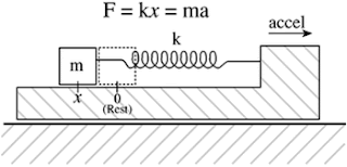
Lets understand the physics of acceleration measurement in Accelerometer using spring and mass systems. Springs generally obey Hooke's law. If this system undergoes an acceleration, then by using Newton's 2nd law and force conserving equation, we get F = ma = kx


F=kx, where k is the constant of proportionality (spring coefficient) between displacement (x) and force (F).
Hence an acceleration a will cause the mass to be displaced by
                                          x=ma/k    -------------- (i) 
alternatively, if we observe a displacement of x, we know that the mass has undergone an acceleration of
                                         a=kx/m      --------------- (ii)

Thus, if we can somehow measure displacement x, we can measure the actual acceleration a on the body.
For accelerometers that use the MEMS technology, two approaches for measuring dominate the market: (i) capacitive sensing, (ii) piezoelectric sensing.

These approaches convert mechanical information into electrical signals by methods that are particular to the silicon technology.
The case of measuring using the capacitive mechanism is considered next
                                                                                                                                                                                                 
A change in causes a change in the capacitance defined by                            
                                   C=ε_0  A/xa                ---------- (iii)
where ε_0 is the permittivity of the air gap, and A is the surface area on either side of the proof mass where the springs are located, xa is the distance between capacitor plate and mass m.
By varying the distance xa , we can vary capacitance ‘C’. Combining Equation  (ii) & (iii), we can find acceleration  ‘a’ in mass ‘m’.
               a=(k.A.ε_0)/mC         --------------- (iv)
This way, you can calculate acceleration in all three axis x, y and z coordinates.
Hope this explination helped many of you to understand the basic physics behind working of accelerometers.

Happy Learning! Please post your comments below :-)